7.4. Negative Streamer Discharge (PIC, Poisson’s Equation)
This test case describes the simulation of streamer formation. Streamers occur when a gas is exposed to high voltages. Streamers occur in lightning and sprites as well as in industrial applications such as lighting, treatment of polluted gases and water, disinfection plasma jets and plasma-assisted combustion. Further optimization and understanding of such applications depend on an accurate knowledge of the electron dynamics during streamer development [37]. For the simulation of a streamer, a neutral gas is seeded with a small number of electrons between two planar electrodes. The evolution follows a well-known pattern: initial electron density increases due to ionization, leading to charge separation as oppositely charged particles drift in the electric field. This distortion of the initially uniform field results in localized screening, eventually halting ionization within the ionized region. As a result, characteristic ionization front profiles of electron and ion densities, as well as the electric field, emerge, marking the transition from an ionization avalanche to a fully developed streamer.
In this tutorial, the streamer formation will be simulated using two different modeling approaches. First, we employ an electron fluid model, where instead of modeling electrons kinetically as particles, their density evolution is described using a fluid approach. However, ions continue to be treated as particles, resulting in a hybrid fluid-kinetic modeling approach (for more details see Section Drift-diffusion model). Next, we simulate the streamer formation using the classical PIC-MCC method (for more details see Section Particle-In-Cell). Finally, both models are compared to evaluate their respective strengths and differences.
7.4.1. Drift-Diffusion Electron Fluid
Before beginning with the tutorial, copy the pic-poisson-streamer from the tutorial folder in the top level directory to a separate location.
cp -r $PICLAS_PATH/tutorials/pic-poisson-streamer .
cd pic-poisson-streamer
For the first part of the tutorial, switch into the drift-diffusion directory via
cd drift-diffusion
before continuing with the mesh building section. Then, the species database needs to be copied into that directory of a symbolic link needs to be created
ln -s $PICLAS_PATH/SpeciesDatabase.h5
7.4.1.1. Mesh Generation with PyHOPE (pre-processing)-1
Before the actual simulation is conducted, a mesh file in the correct HDF5 format has to be supplied. The mesh files used by piclas are created by supplying an input file hopr.ini with the required information for a mesh that has either been created by an external mesh generator or directly from block-structured information in the hopr.ini file itself. Here, a block-structured grid is created directly from the information in the hopr.ini file.
To create the .h5 mesh file, simply run
pyhope hopr.ini
This creates the mesh file streamer_mesh.h5 in HDF5 format. Alternatively, if you do not want to run PyHOPE yourself, you can also use the provided mesh. The only difference from the mesh created in previous tutorial, is the size of the simulation domain in this tutorial which is set to [\(4\pi\times1\times1\)] m\(^{3}\) and is defined by the single block information
in the line, where each node of the hexahedral element is defined. Here, l1 and l2 define the dimensions of the hexahedral elements. While l1 represents the length in the x-direction, l2 indicates the length in the y-direction.
Corner = (/0.,0.,0.,,l1,0.,0.,,l1,l2,0.,,0.,l2,0.,,0.,0.,l2,,l1,0.,l2,,l1,l2,l2,,0.,l2,l2/)
The number of mesh elements for the block in each direction can be adjusted by changing the line. ni defines the number of elements to be created in the x-direction. This allows for adjusting the number of elements within a block.
nElems = (/ni,1,1/) ! number of elements in each direction
Each side of the block has to be assigned a boundary index, which corresponds to the boundaries defined in the next steps
BCIndex = (/5,3,2,4,1,6/) ! Indices of UserDefinedBoundaries
The field boundaries can directly be defined in the hopr.ini file (contrary to the particle boundary conditions, which are defined in the parameter.ini). Periodic boundaries should be defined in the hopr.ini.
!=============================================================================== !
! BOUNDARY CONDITIONS
!=============================================================================== !
BoundaryName = BC_Xleft
BoundaryType = (/3,0,0,0/)
BoundaryName = BC_Xright
BoundaryType = (/3,0,0,0/)
BoundaryName = BC_periodicy+ ! Periodic (+vv1)
BoundaryType = (/1,0,0,1/)   ! Periodic (+vv1)
BoundaryName = BC_periodicy- ! Periodic (-vv1)
BoundaryType = (/1,0,0,-1/)  ! Periodic (-vv1)
BoundaryName = BC_periodicz+ ! Periodic (+vv2)
BoundaryType = (/1,0,0,2/)   ! Periodic (+vv2)
BoundaryName = BC_periodicz- ! Periodic (-vv2)
BoundaryType = (/1,0,0,-2/)  ! Periodic (-vv2)

VV=(/0. , l2 , 0./)    ! Displacement vector 1 (y-direction)
VV=(/0. , 0. , l2/)   ! Displacement vector 2 (z-direction)
7.4.1.2. Simulation with PICLas-1
Install piclas by compiling the source code as described in Chapter Installation, specifically described under Section Compiling the code. Always build the code in a separate directory located in the piclas top level directory. For this PIC tutorial, e.g., create a directory build_drift_diffusion by running
cd $PICLAS_PATH
where the variable PICLAS_PATH contains the path to the location of the piclas repository and the create the build directory, in which the compilation process will take place. This command should be run in the piclas folder.
mkdir build_drift_diffusion
Always compile the code within the build directory, hence, navigate to the build_drift_diffusion directory before running cmake
cd build_drift_diffusion
For this specific tutorial, make sure to set the correct compile flags
PICLAS_EQNSYSNAME       = drift_diffusion
LIBS_USE_PETSC          = ON
PICLAS_READIN_CONSTANTS = ON
PICLAS_TIMEDISCMETHOD   = Explicit-FV
using the ccmake (gui for cmake) or simply run the following command from inside the build directory
cmake .. -DPICLAS_EQNSYSNAME=drift_diffusion -DPICLAS_TIMEDISCMETHOD=Explicit-FV -DLIBS_USE_PETSC=ON
to configure the build process and run
make -j
afterwards to compile the executable. For this setup, we have chosen the drift_diffusion solver and selected the Explicit-FV time discretization method. An overview over the available solver and discretization options is given in Section Solver settings. To run the simulation and analyse the results, the piclas and piclas2vtk executables have to be run. To avoid having to use the entire file path, you can either set aliases for both, copy them to your local tutorial directory or create a link to the files via
ln -s $PICLAS_PATH/build_drift_diffusion/bin/piclas
ln -s $PICLAS_PATH/build_drift_diffusion/bin/piclas2vtk
where the variable PICLAS_PATH contains the path to the location of the piclas repository.
7.4.1.2.1. General numerical setup-1
The general numerical parameters (defined in the parameter.ini) are selected by the following
! =============================================================================== !
! DISCRETIZATION
! =============================================================================== !
N             = 1  ! Polynomial degree of the DG method (field solver)

! =============================================================================== !
! MESH
! =============================================================================== !
MeshFile      = ./streamer_mesh.h5 ! Relative path to the mesh .h5 file

! =============================================================================== !
! General
! =============================================================================== !
ProjectName       = streamer_N2
doPrintStatusLine = T                   ! Output live of ETA
where, among others, the polynomial degree \(N\), the path to the mesh file MeshFile, project name and the option to print the ETA
to the terminal output in each time step.
The temporal parameters of the simulation are controlled via
! =============================================================================== !
! CALCULATION
! =============================================================================== !
ManualTimeStep  = 1.e-13
tend            = 7.e-10
Analyze_dt      = 0.5e-10
IterDisplayStep = 100
where the time step for the field and particle solver is set via ManualTimeStep, the final simulation time tend, the time
between restart/checkpoint file output Analyze_dt (also the output time for specific analysis functions) and the number of time
step iterations IterDisplayStep between information output regarding the current status of the simulation that is written to std.out.
The remaining parameters are selected for the field and particle solver as well as run-time analysis.
7.4.1.2.2. Boundary conditions-1
As there are no walls present in the setup, all boundaries are set as periodic boundary conditions for the field as well as the particle solver. The particle boundary conditions are set by the following lines
! =============================================================================== !
! PARTICLE Boundary Conditions
! =============================================================================== !
Part-nBounds              = 6             ! Number of particle boundaries
Part-Boundary1-SourceName = BC_Xleft      ! Name of 1st particle BC
Part-Boundary1-Condition  = symmetric     ! Type of 1st particle BC
Part-Boundary2-SourceName = BC_Xright     ! ...
Part-Boundary2-Condition  = symmetric     ! ...
Part-Boundary3-SourceName = BC_periodicy+ ! ...
Part-Boundary3-Condition  = periodic      ! ...
Part-Boundary4-SourceName = BC_periodicy- ! ...
Part-Boundary4-Condition  = periodic      ! ...
Part-Boundary5-SourceName = BC_periodicz+ ! ...
Part-Boundary5-Condition  = periodic      ! ...
Part-Boundary6-SourceName = BC_periodicz- ! ...
Part-Boundary6-Condition  = periodic      ! ...

Part-nPeriodicVectors = 2 ! Number of periodic boundary (particle and field) vector
7.4.1.2.3. Field solver-1
The settings for the field solver (HDGSEM) are given by
! =============================================================================== !
! Field Solver: HDGSEM
! =============================================================================== !
epsCG                 = 1e-6   ! Stopping criterion (residual) of iterative CG solver (default that is used for the HDGSEM solver)
maxIterCG             = 10000  ! Maximum number of iterations
IniExactFunc          = 0      ! Initial field condition. 0: zero solution vector
where epsCG sets the abort residual of the CG solver, maxIterCG sets the maximum number of iterations within the CG solver and
IniExactFunc set the initial solution of the field solver (here 0 says that nothing is selected). Also the initial solution of the
electron fluid solver must be set by
! =============================================================================== !
! Electron Fluid
! =============================================================================== !

IniExactFunc-FV  = 3  !streamer
IniRefState-FV   = 1

RefState-FV=(/2.e18/)

Grad-LimiterType = 0
The IniExactFunc-FV is set to 3, as this represents a special initial condition for the streamer test case.
Here, a Gaussian-type distribution of electrons is initialized at x = 0.8 mm.
The maximum number density is defined by RefState-FV.
The numerical scheme for tracking the movement of all particles throughout the simulation domain can be switched by
! =============================================================================== !
! Particle Solver
! =============================================================================== !
TrackingMethod    = triatracking ! Particle tracking method
The PIC parameters for interpolation (of electric fields to the particle positions) and deposition (mapping of charge properties from particle locations to the grid) are selected via
! =============================================================================== !
! PIC: Interpolation/Deposition
! =============================================================================== !
PIC-DoInterpolation            = T                        ! Activate Lorentz forces acting on charged particles
PIC-Interpolation-Type         = particle_position        ! Field interpolation method for Lorentz force calculation
PIC-Deposition-Type            = cell_volweight_mean
PIC-shapefunction-radius       = 0.0001
PIC-shapefunction-dimension    = 1                        ! Shape function specific dimensional setting
where the interpolation type PIC-Interpolation-Type = particle_position is currently the only option for specifying how
electro(-magnetic) fields are interpolated to the position of the charged particles.
The dimension PIC-shapefunction-dimension, here 1D and direction PIC-shapefunction-direction, are selected specifically
for the one-dimensional setup that is simulated here. The different available deposition types are described in more detail in Section Charge and Current Deposition.
7.4.1.2.4. Particle solver-1
For the treatment of particles, the maximum number of particles Part-maxParticleNumber that each processor can hold has to be supplied and
the number of particle species Part-nSpecies that are used in the simulation (created initially or during the simulation time
through chemical reactions).
! =============================================================================== !
! PARTICLE Emission
! =============================================================================== !
Particles-Species-Database = SpeciesDatabase.h5
Part-nSpecies             = 2        ! Number of particle species


! -------------------------------------
! Background Gas - N2
! -------------------------------------
Part-Species1-SpeciesName = N2
Part-Species1-MacroParticleFactor       = 1500.
BGGas-DriftDiff-Database = Phelps


Part-Species1-nInits                      = 1

Part-Species1-Init1-velocityDistribution  = maxwell_lpn
Part-Species1-Init1-SpaceIC               = background
Part-Species1-Init1-PartDensity           = 2.506e25
Part-Species1-Init1-VeloIC                = 0.
Part-Species1-Init1-VeloVecIC             = (/1.,0.,0./)
Part-Species1-Init1-MWTemperatureIC       = 298.
Part-Species1-Init1-TempVib               = 298.
Part-Species1-Init1-TempRot               = 298.
Part-Species1-Init1-TempElec              = 298.

! -------------------------------------
! Ions - N2+
! -------------------------------------
Part-Species2-SpeciesName = N2Ion1
Part-Species2-MacroParticleFactor = 1500. ! Weighting factor for species #2
Part-Species2-nInits              = 0               ! Number of initialization/emission regions for species #1

Particles-HaloEpsVelo = 3.E8
7.4.1.2.5. Field Boundaries-1
BoundaryName specifies the name of the boundary. Two boundaries are defined here: BC_Xleft (left x boundary) and BC_Xright (right x boundary). BoundaryType defines the type of boundary condition. Each BoundaryType is expressed as a pair of numbers, such as ((/12,0/), (/4,0/)). ‘12’ represents a Neumann boundary condition, which defines a situation where the electric field (E) remains constant. ‘4’ represents a Dirichlet boundary condition, indicating a situation where the potential is zero (for example, a grounded surface). ‘11’ defines a special type of Neumann boundary condition. In this case, it represents conditions where the electric field (E) has a constant value, but unlike number 12, ‘11’ includes a more specific condition.
! =============================================================================== !
! Field Boundaries
! =============================================================================== !
BoundaryName = BC_Xleft
BoundaryType = (/12,0/)   ! 12: Neumann with fixed E = -1.45e7 V/m
BoundaryType-FV = (/3,0/) ! Neumann for eFluid


BoundaryName = BC_Xright
BoundaryType = (/4,0/) ! 4: Dirichlet with zero potential
BoundaryType-FV = (/3,0/) ! Neumann for eFluid
7.4.1.2.6. Analysis setup-1
Finally, some parameters for run-time analysis are chosen by setting them T (true). Further, with TimeStampLength = 18, the names of the output files are shortened for better postprocessing. If this is not done, e.g. Paraview does not sort the files correctly and will display faulty behaviour over time.
! =============================================================================== !
! Analysis
! =============================================================================== !
TimeStampLength          = 18 ! Reduces the length of the timestamps in filenames for better postprocessing
CalcCharge               = T  ! writes rel/abs charge error to PartAnalyze.csv
CalcPotentialEnergy      = T  ! writes the potential field energy to FieldAnalyze.csv
CalcKineticEnergy        = T  ! writes the kinetic energy of all particle species to PartAnalyze.csv
PIC-OutputSource         = T  ! writes the deposited charge (RHS of Poissons equation to XXX_State_000.0000XXX.h5)
CalcPICTimeStep          = T  ! writes the PIC time step restriction to XXX_State_000.0000XXX.h5 (rule of thumb)
CalcPointsPerDebyeLength = T  ! writes the PIC grid step restriction to XXX_State_000.0000XXX.h5 (rule of thumb)
CalcTotalEnergy          = T  ! writes the total energy of the system to PartAnalyze.csv (field and particle)

CalcElectronTemperature = T
CalcDebyeLength = T
CalcPlasmaFrequency = T
The function of each parameter is given in the code comments. Information regarding every parameter can be obtained from running the command
piclas --help "CalcCharge"
where each parameter is simply supplied to the help module of piclas. This help module can also output the complete set of
parameters via piclas --help or a subset of them by supplying a section, e.g., piclas --help "HDG" for the HDGSEM solver.
7.4.1.2.7. Running the code-1
The command
./piclas parameter.ini | tee std.out
executes the code and dumps all output into the file std.out.
If the run has completed successfully, which should take only a brief moment, the contents of the working folder should look like
8.0K -rw-rw-r--  5.8K *** 28 12:51 ElemTimeStatistics.csv
120K -rw-rw-r--  113K *** 28 12:51 FieldAnalyze.csv
4.0K -rw-rw-r--  2.1K *** 26 16:49 hopr.ini
8.0K -rw-rw-r--  5.0K *** 28 13:07 parameter_streamer.ini
156K -rw-rw-r--  151K *** 28 12:51 PartAnalyze.csv
 32K -rw-rw-r--   32K *** 26 16:43 streamer_N2_mesh.h5
1.6M -rw-rw-r--  1.6M *** 28 12:44 streamer_N2_DSMCState_000.00000000001000.h5
1.6M -rw-rw-r--  1.6M *** 28 12:45 streamer_N2_DSMCState_000.00000000002000.h5
1.6M -rw-rw-r--  1.6M *** 28 12:45 streamer_N2_DSMCState_000.00000000003000.h5
1.6M -rw-rw-r--  1.6M *** 28 12:46 streamer_N2_DSMCState_000.00000000004000.h5
1.6M -rw-rw-r--  1.6M *** 28 12:47 streamer_N2_DSMCState_000.00000000005000.h5
1.6M -rw-rw-r--  1.6M *** 28 12:48 streamer_N2_DSMCState_000.0000000000****.h5
1.6M -rw-rw-r--  1.6M *** 28 12:49 streamer_N2_DSMCState_000.0000000000****.h5
1.6M -rw-rw-r--  1.6M *** 28 12:50 streamer_N2_DSMCState_000.0000000000****.h5
1.6M -rw-rw-r--  1.6M *** 28 12:50 streamer_N2_DSMCState_000.0000000000****.h5
1.6M -rw-rw-r--  1.6M *** 28 12:51 streamer_N2_State_000.00000000099000.h5
1.6M -rw-rw-r--  1.6M *** 28 12:51 streamer_N2_State_000.00000000100000.h5
 72K -rw-rw-r--   71K *** 28 12:51 std.out
Multiple additional files have been created, which are are named Projectname_State_Timestamp.h5.
They contain the solution vector of the equation system variables at each interpolation nodes at the given time, which corresponds
to multiples of Analyze_dt. If these files are not present, something went wrong during the execution of piclas.
In that case, check the std.out file for an error message.
After a successful completion, the last lines in this file should look as shown below:
====================================================================================================================================
PICLAS FINISHED! [ #######.## sec ] [ #:##:##:## ]
====================================================================================================================================
7.4.1.3. Visualization (post-processing)-1
To visualize the solution, the State-files must be converted into a format suitable for ParaView, VisIt or any other visualisation tool for which the program piclas2vtk is used.
The parameters for piclas2vtk are stored in the parameter.ini file under
! =============================================================================== !
! piclas2vtk
! =============================================================================== !
NVisu         = 1 ! Polynomial degree used for the visualization when the .h5 file is converted to .vtu/.vtk format. Should be at least N+1
VisuParticles = F  ! Activate the conversion of particles from .h5 to .vtu/.vtk format. Particles will be displayed as a point cloud with properties, such as velocity, species ID, etc.

Part-NumberOfRandomSeeds = 2
Particles-RandomSeed1    = 1
Particles-RandomSeed2    = 2
where NVisu is the polynomial visualization degree on which the field solution is interpolated.
Depending on the used polynomial degree N, the degree of visualization NVisu should always be higher than
N because the PIC simulation is always subject to noise that is influenced by the discretization (number of elements and
polynomial degree as well as number of particles) and is visible in the solution results of the current simulation.
Additionally, the flag VisuParticles activates the output of particle position, velocity and species to the vtk-files.
Run the command
./piclas2vtk parameter.ini streamer_N2_State_000.00000000*
to generate the corresponding vtk-files, which can then be loaded into the visualisation tool.
The electron and ion densities (streamer_N2_Solution_ElemData_000.00* at t=0 s, t=0.35 ns and t=0.7 ns) and electric field in x-direction (streamer_N2_Solution_000.00000000070000.vtu) at t=0.7 ns (end of simulation) are shown in the plots.
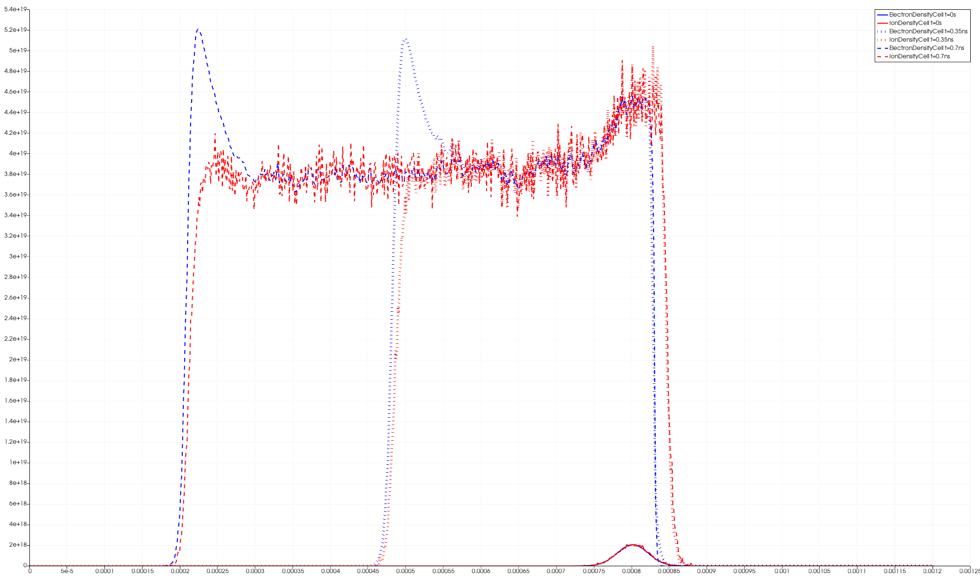
Fig. 7.7 Electron and ion density in a planar front in nitrogen gas.

Fig. 7.8 Electric Field across the domain.
7.4.2. Particle-in-cell/Monte Carlo Collision (PIC/MCC)
In this tutorial, we extend the concepts introduced in the fluid-based streamer simulation to a fully kinetic particle model using the Particle-in-Cell (PIC) method combined with Monte Carlo Collisions (MCC). Unlike the fluid model, which uses a macroscopic description of electron transport, the PIC-MCC model resolves the motion and collisions of individual particles, enabling detailed modeling of ionization and streamer dynamics in nitrogen gas. This tutorial demonstrates how to simulate a negative streamer discharge using the Particle-in-Cell (PIC) with Monte Carlo Collision (MCC) model in PICLas. The simulation setup largely mirrors the structure used in the fluid case, and only the key differences will be described here. For general steps such as mesh generation and basic solver configuration, please refer to the corresponding sections in the fluid-based tutorial.
Before beginning the tutorial, go back to the parent directory pic-poisson-streamer that you copied from the tutorial folder at the beginning of the tutorial. For the second part of the tutorial, switch now into the pic-mcc directory
cd pic-mcc
before continuing with the mesh building section. Then again, the species database needs to be within that directory, so a symbolic link needs to be created
ln -s $PICLAS_PATH/SpeciesDatabase.h5
In addition, an electronic database is needed. This can be linked or copied from one of the regressionchecks, e.g.
cp $PICLAS_PATH/regressioncheck/NIG_Reservoir/MCC_BGG_MultiSpec_XSec_TCE_QK_Chem/DSMCSpecies_electronic_state_full_Data.h5 .
7.4.2.1. Mesh Generation with PyHOPE (pre-processing)-2
The mesh generation process is identical to that described in the fluid model section. Please refer to that section for detailed instructions or you just copy the mesh from the previous part of the tutorial
cp ../drift-diffusion/streamer_mesh.h5 ./
7.4.2.2. Simulation with PICLas-2
Install piclas by compiling the source code as described in Chapter Installation, specifically described under Section Compiling the code. Always build the code in a separate directory located in the piclas top level directory. For this PIC tutorial, e.g., create a directory build_poisson_Leapfrog by running
cd $PICLAS_PATH
where the variable PICLAS_PATH contains the path to the location of the piclas repository and the create the build directory, in which the compilation process will take place. This command should be run in the piclas folder.
mkdir build_poisson_Leapfrog
Always compile the code within the build directory, hence, navigate to the build_poisson_Leapfrog directory before running cmake
cd build_poisson_Leapfrog
For this specific tutorial, make sure to set the correct compile flags
PICLAS_EQNSYSNAME     = poisson
LIBS_USE_PETSC        = ON
PICLAS_TIMEDISCMETHOD = Leapfrog
using the ccmake (gui for cmake) or simply run the following command from inside the build directory
cmake ../ -DPICLAS_EQNSYSNAME=poisson -DPICLAS_TIMEDISCMETHOD=Leapfrog -DLIBS_USE_PETSC=ON
to configure the build process and run
make -j
afterwards to compile the executable. For this setup, we have chosen the Poisson solver and selected the Leapfrog time discretization method. An overview over the available solver and discretization options is given in Section Solver settings. To run the simulation and analyse the results, the piclas and piclas2vtk executables have to be run. To avoid having to use the entire file path, you can either set aliases for both, copy them to your local tutorial directory or create a link to the files via
ln -s $PICLAS_PATH/build_poisson_Leapfrog/bin/piclas
ln -s $PICLAS_PATH/build_poisson_Leapfrog/bin/piclas2vtk
where the variable PICLAS_PATH contains the path to the location of the piclas repository.
7.4.2.2.1. General numerical setup-2
The general numerical parameters (defined in the parameter.ini) are selected by the following
! =============================================================================== !
! DISCRETIZATION
! =============================================================================== !
N             = 2  ! Polynomial degree of the DG method (field solver)

! =============================================================================== !
! MESH
! =============================================================================== !
MeshFile      = streamer_mesh.h5 ! Relative path to the mesh .h5 file

! =============================================================================== !
! General
! =============================================================================== !
ProjectName       = streamer_N2 ! Project name that is used for naming state files
ColoredOutput     = F           ! Turn ANSI terminal colors ON/OFF
doPrintStatusLine = T           ! Output live of ETA
TrackingMethod    = TriaTracking
where, among others, the polynomial degree \(N\), the path to the mesh file MeshFile, project name and the option to print the ETA
to the terminal output in each time step.
The temporal parameters of the simulation are controlled via
! =============================================================================== !
! CALCULATION
! =============================================================================== !
ManualTimeStep                   = 1e-13  ! Fixed pre-defined time step only when using the Poisson solver. Maxwell solver calculates dt that considers the CFL criterion
tend                             = 7e-10  ! Final simulation time
Analyze_dt                       = 5E-12  ! decrease analyze_dt for better resolution of fish eye
IterDisplayStep                  = 500    ! Number of iterations between terminal output showing the current time step iteration
Part-WriteMacroValues            = T      ! Set [T] to activate ITERATION DEPENDANT h5 output of macroscopic values sampled (Can not be enabled together with Part-TimeFracForSampling)
Part-IterationForMacroVal        = 100    ! Set number of iterations used for sampling                                      (Can not be enabled together with Part-TimeFracForSampling)
where the time step for the field and particle solver is set via ManualTimeStep, the final simulation time tend, the time
between restart/checkpoint file output Analyze_dt (also the output time for specific analysis functions) and the number of time
step iterations IterDisplayStep between information output regarding the current status of the simulation that is written to std.out.
The remaining parameters are selected for the field and particle solver as well as run-time analysis.
7.4.2.2.2. Boundary conditions-2
As there are no walls present in the setup, all boundaries are set as periodic boundary conditions for the field as well as the particle solver. The particle boundary conditions are set by the following lines
! =============================================================================== !
! PARTICLE Boundary Conditions
! =============================================================================== !
Part-nBounds              = 6             ! Number of particle boundaries
Part-Boundary1-SourceName = BC_Xleft      ! Name of 1st particle BC
Part-Boundary1-Condition  = symmetric     ! Type of 1st particle BC
Part-Boundary2-SourceName = BC_Xright     ! ...
Part-Boundary2-Condition  = symmetric     ! ...
Part-Boundary3-SourceName = BC_periodicy+ ! ...
Part-Boundary3-Condition  = periodic      ! ...
Part-Boundary4-SourceName = BC_periodicy- ! ...
Part-Boundary4-Condition  = periodic      ! ...
Part-Boundary5-SourceName = BC_periodicz+ ! ...
Part-Boundary5-Condition  = periodic      ! ...
Part-Boundary6-SourceName = BC_periodicz- ! ...
Part-Boundary6-Condition  = periodic      ! ...

Part-nPeriodicVectors = 2 ! Number of periodic boundary (particle and field) vectors
7.4.2.2.3. Field solver-2
The settings for the field solver (HDGSEM) are given by
! =============================================================================== !
! Field Solver: HDGSEM
! =============================================================================== !
epsCG                 = 1e-6   ! Stopping criterion (residual) of iterative CG solver (default that is used for the HDGSEM solver)
maxIterCG             = 10000  ! Maximum number of iterations
IniExactFunc          = 0      ! Initial field condition. 0: zero solution vector
PrecondType           = 2
For this tutroial we use a PETSc Solver where a multitude of different numerical methods to solve the resulting system of linear equations is given by the implemented PETSc library and epsCG sets the abort residual of the CG solver, maxIterCG sets the maximum number of iterations within the CG solver, the PrecondType is set to 2, IniExactFunc sets the initial solution of the field solver (here 0 says that nothing is selected).
The PIC parameters for interpolation (of electric fields to the particle positions) and deposition (mapping of charge properties from particle locations to the grid) are selected via
! =============================================================================== !
! PIC: Interpolation/Deposition
! =============================================================================== !
PIC-DoInterpolation      = T                   ! Activate Lorentz forces acting on charged particles
PIC-Interpolation-Type   = particle_position   ! Field interpolation method for Lorentz force calculation

PIC-Deposition-Type      = cell_volweight_mean ! Linear deposition method
where the interpolation type PIC-Interpolation-Type = particle_position is currently the only option for specifying how
electro(-magnetic) fields are interpolated to the position of the charged particles.
For charge and current deposition,
PIC-Deposition-Type = cell_volweight_mean is selected.
The different available deposition types are described in more detail in Section Charge and Current Deposition.
7.4.2.2.4. Particle solver-2
The numerical scheme for tracking the movement of all particles throughout the simulation domain can be switched by
! =============================================================================== !
! Particle Solver
! =============================================================================== !
TrackingMethod    = triatracking ! Particle tracking method
For the treatment of particles, the number of particle species Part-nSpecies that are used in the simulation (created initially or during the simulation time
through chemical reactions).
! =============================================================================== !
! PARTICLE Emission
! =============================================================================== !
Part-nSpecies             = 3    ! Number of particle species
In contrast to the fluid case, PICLas does not allow specifying a local Gaussian distribution for the spatial distribution of the initial electrons and ions as particles. Therefore, the initial particles are uniformly distributed within a cubic volume centered at x = 0.8 mm, in order to create initial conditions similar to those in the fluid case. As in the fluid case, neutral molecular nitrogen N2 is not represented by particles but defined as a background gas. The definition of the initial condition for all species in the ini-file is as follows:
! =============================================================================== !
! Background Gas - N2
! =============================================================================== !
Part-Species1-MacroParticleFactor       = 200
Part-Species1-nInits                      = 1
Part-Species1-Init1-velocityDistribution  = maxwell_lpn
Part-Species1-Init1-SpaceIC               = background
Part-Species1-Init1-PartDensity           = 2.506e25
Part-Species1-Init1-VeloIC                = 0.
Part-Species1-Init1-VeloVecIC             = (/1.,0.,0./)
Part-Species1-Init1-MWTemperatureIC       = 298.
Part-Species1-Init1-TempVib               = 298.
Part-Species1-Init1-TempRot               = 298.
! =============================================================================== !
! Ions - N2+
! =============================================================================== !
!Part-Species2-SpeciesName = N2Ion1
Part-Species2-MacroParticleFactor = 200         ! Weighting factor for species #2
Part-Species2-nInits              = 1           ! Number of initialization/emission regions for species #1
Part-Species2-Init1-SpaceIC               = cuboid   !(cartesian)
Part-Species2-Init1-ParticleNumber        = 1000   ! 1000*200/(5e-5)^3 => 1.6e18
Part-Species2-Init1-BasePointIC           =(/0.000775 , 0. , 0./)
Part-Species2-Init1-BaseVector1IC         =(/0, 0.00005 , 0./)
Part-Species2-Init1-BaseVector2IC         =(/0, 0. , 0.00005/)
Part-Species2-Init1-NormalIC              =(/1, 0. , 0./)
Part-Species2-Init1-CuboidHeightIC        = 0.00005
Part-Species2-Init1-velocityDistribution  = maxwell_lpn !constant( unrealistic temp)
Part-Species2-Init1-MWTemperatureIC       = 298.
Part-Species2-Init1-TempVib               = 298.
Part-Species2-Init1-TempRot               = 298.
! =============================================================================== !
!  Electrons 1
! =============================================================================== !
Part-Species3-MacroParticleFactor         = 200
Part-Species3-nInits                      = 1
Part-Species3-Init1-SpaceIC               = cuboid   !(cartesian)
Part-Species3-Init1-ParticleNumber        = 1000   ! 1000*200/(5e-5)^3 => 1.6e18
Part-Species3-Init1-BasePointIC           =(/0.000775 , 0. , 0./)
Part-Species3-Init1-BaseVector1IC         =(/0, 0.00005 , 0./)
Part-Species3-Init1-BaseVector2IC         =(/0, 0. , 0.00005/)
Part-Species3-Init1-NormalIC              =(/1, 0. , 0./)
Part-Species3-Init1-CuboidHeightIC        = 0.00005
Part-Species3-Init1-velocityDistribution  = maxwell_lpn !constant( unrealistic temp)
Part-Species3-Init1-MWTemperatureIC       = 298
Each initialization set is accompanied by a block of parameters that is preceded by the corresponding -Init[$] counter. The Part-Species[$]-Init[$]-SpaceIC = cuboid flag defines the type of the initialization set. Here, the particles are placed in a cuboid which is spanned by its base plane (Part-Species[$]-Init[$]-BasePointIC, Part-Species[$]-Init[$]-BaseVector1IC, Part-Species[$]-Init[$]-BaseVector2IC), a normal (Part-Species[$]-Init[$]-NormalIC) and its height (Part-Species[$]-Init[$]-CuboidHeightIC). Each type of the initialization set might have a different set of parameters and an overview is given in Section
Particle Initialization & Emission.
In order to reduce the simulation time we use the flag
Part-vMPF                           = T
Part-Species2-vMPFMergeThreshold    = 300
Part-Species3-vMPFMergeThreshold    = 300
The merge routine randomly deletes particles until the desired number of particles is reached and the weighting factor is adopted accordingly.
Since we are dealing with ionization reaction in this setup, DSMC has to be enabled (UseDSMC = T). Particles-DSMC-CollisMode is an important parameterwhich has to beset to 3 so that chemistry is enabled.
!===============================================================================
! DSMC
!===============================================================================
UseDSMC                           = T
Particles-DSMC-CollisMode         = 3
After the chemistry is enabled, the model for a reaction has to be chosen. In our setup, it would be the cross section collision model. We only have one ionization reaction due to collision occuring in our setup $\( e^- + N_2 \rightarrow 2e^- + N_2^+ \)$ we will then define the reaction by
DSMC-NumOfReactions                       = 1
DSMC-Reaction1-ReactionModel              = XSec
DSMC-Reaction1-Reactants                  = (/1,3,0/)
DSMC-Reaction1-Products                   = (/2,3,3,0/)
For more information regarding different chemistry models refer to the section Chemistry & Ionization.
As we are dealing with a particle model of the streamer case for modelling of particle collisions with the Particle-in-Cell method, often the Monte Carlo Collision (MCC) algorithm is utilized. Here, experimentally measured or ab-initio calculated cross-sections are typically utilized to determine the collision probability, based on the cross-section [m\(^2\)], the timestep [s], the particle velocity [m/s] and the target gas number density [m\(^{-3}\)]. To activate the MCC procedure, the collision cross-sections have to be supplied via read-in from a database.
Particles-CollXSec-Database               = XSec_Database_N2_Ionized.h5
Particles-CollXSec-NullCollision          = T
In PICLas, the null collision method reduces the computational effort as not every particle has to be checked for a collision. Cross-section data can be retrieved from the LXCat database and converted with a Python script provided in the tools folder: piclas/tools/crosssection_database. Refer to the section Collision cross-sections for more information.
For more information regarding cross-section based collision probability refer to the section Background Gas.
7.4.2.2.5. Field Boundaries-2
To accelarate the electrons towards the left boundary of the domain, i.e x=0, external electric field is provided.
! =============================================================================== !
! Field Boundaries
! =============================================================================== !
BoundaryName = BC_Xleft
BoundaryType = (/12,0/)                ! Neumann with fixed E = -1.45e7 V/m

BoundaryName = BC_Xright
BoundaryType = (/4,0/)                 ! 4: Dirichlet with zero potential
7.4.2.2.6. Analysis setup-2
Finally, some parameters for run-time analysis are chosen by setting them T (true). Further, with TimeStampLength = 18, the names of the output files are shortened for better postprocessing. If this is not done, e.g. Paraview does not sort the files correctly and will display faulty behaviour over time.
! =============================================================================== !
! Analysis
! =============================================================================== !
TimeStampLength          = 18 ! Reduces the length of the timestamps in filenames for better postprocessing
CalcCharge               = T ! writes rel/abs charge error to PartAnalyze.csv
CalcPotentialEnergy      = T ! writes the potential field energy to FieldAnalyze.csv
CalcKineticEnergy        = T ! writes the kinetic energy of all particle species to PartAnalyze.csv
PIC-OutputSource         = T ! writes the deposited charge (RHS of Poisson's equation to XXX_State_000.0000XXX.h5)
CalcPICTimeStep          = T ! writes the PIC time step restriction to XXX_State_000.0000XXX.h5 (rule of thumb)
CalcPointsPerDebyeLength = T ! writes the PIC grid step restriction to XXX_State_000.0000XXX.h5 (rule of thumb)
CalcTotalEnergy          = T ! writes the total energy of the system to PartAnalyze.csv (field and particle)
CalcInternalEnergy       = T
CalcElectronTemperature  = T
CalcDebyeLength          = T
CalcPlasmaFrequency      = T
CalcNumDens              = T
CalcNumSpec              = T
The function of each parameter is given in the code comments. Information regarding every parameter can be obtained from running the command
piclas --help "CalcCharge"
where each parameter is simply supplied to the help module of piclas. This help module can also output the complete set of
parameters via piclas --help or a subset of them by supplying a section, e.g., piclas --help "HDG" for the HDGSEM solver.
7.4.2.2.7. Running the code-2
The command
./piclas parameter.ini DSMC.ini | tee std.out
executes the code and dumps all output into the file std.out. To reduce the computation time, the simulation can be run using the Message Passing Interface (MPI) on multiple cores, in this case 8
mpirun -np 8 piclas parameter.ini | tee std.out
If the run has completed successfully, which should take only a brief moment, the contents of the working folder should look like
4.0K drwxrwxr-x  4.0K Jun 28 13:07 ./
4.0K drwxrwxr-x  4.0K Jun 25 23:56 ../
8.0K -rw-rw-r--  5.8K Jun 28 12:51 ElemTimeStatistics.csv
120K -rw-rw-r--  113K Jun 28 12:51 FieldAnalyze.csv
4.0K -rw-rw-r--  2.1K Jun 26 16:49 hopr.ini
8.0K -rw-rw-r--  5.0K Jun 28 13:07 parameter.ini
156K -rw-rw-r--  151K Jun 28 12:51 PartAnalyze.csv
 32K -rw-rw-r--   32K Jun 26 16:43 streamer_mesh.h5
1.6M -rw-rw-r--  1.6M Jun 28 12:44 streamer_N2_State_000.00000000000000.h5
......
1.6M -rw-rw-r--  1.6M Jun 28 12:51 streamer_N2_State_000.00000000100000.h5

1.6M -rw-rw-r--  1.6M Jun 28 12:51 streamer_N2_DSMCState_000.00000000001000.h5
.......
1.6M -rw-rw-r--  1.6M Jun 28 12:51 streamer_N2_DSMCState_000.00000000100000.h5

72K -rw-rw-r--   71K Jun 28 12:51 std.out
Multiple additional files have been created, which are are named Projectname_State_Timestamp.h5.
They contain the solution vector of the equation system variables at each interpolation nodes at the given time, which corresponds
to multiples of Analyze_dt. If these files are not present, something went wrong during the execution of piclas.
In that case, check the std.out file for an error message.
After a successful completion, the last lines in this file should look as shown below:
====================================================================================================================================
PICLAS FINISHED! [ #######.## sec ] [ #:##:##:## ]
====================================================================================================================================
7.4.2.3. Visualization (post-processing)-2
To visualize the solution, the State-files must be converted into a format suitable for ParaView, VisIt or any other visualisation tool for which the program piclas2vtk is used.
The parameters for piclas2vtk are stored in the parameter.ini file under
! =============================================================================== !
! piclas2vtk
! =============================================================================== !
NVisu         = 3! Polynomial degree used for the visualization when the .h5 file is converted to .vtu/.vtk format. Should be at least N+1
VisuParticles = T  ! Activate the conversion of particles from .h5 to .vtu/.vtk format. Particles will be displayed as a point cloud with properties, such as velocity, species ID, etc.
where NVisu is the polynomial visualization degree on which the field solution is interpolated.
Depending on the used polynomial degree N and subsequently the degree of visualization NVisu, which should always be higher than
N.
Additionally, the flag VisuParticles activates the output of particle position, velocity and species to the vtk-files.
Run the command
./piclas2vtk parameter.ini streamer_N2_State_000.00000000*
to generate the corresponding vtk-files, which can then be loaded into the visualisation tool.
The electron and ion densities (streamer_N2_Solution_ElemData_000.00* at t=0 s, t=0.35 ns and t=0.7 ns) and electric field in x-direction (streamer_N2_Solution_000.00000000070000.vtu) at t=0.7 ns (end of simulation) are shown in the plots.
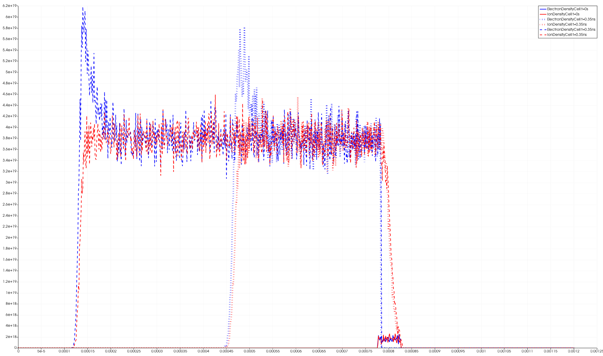
Fig. 7.9 Electron and ion density in a planar front in nitrogen gas.
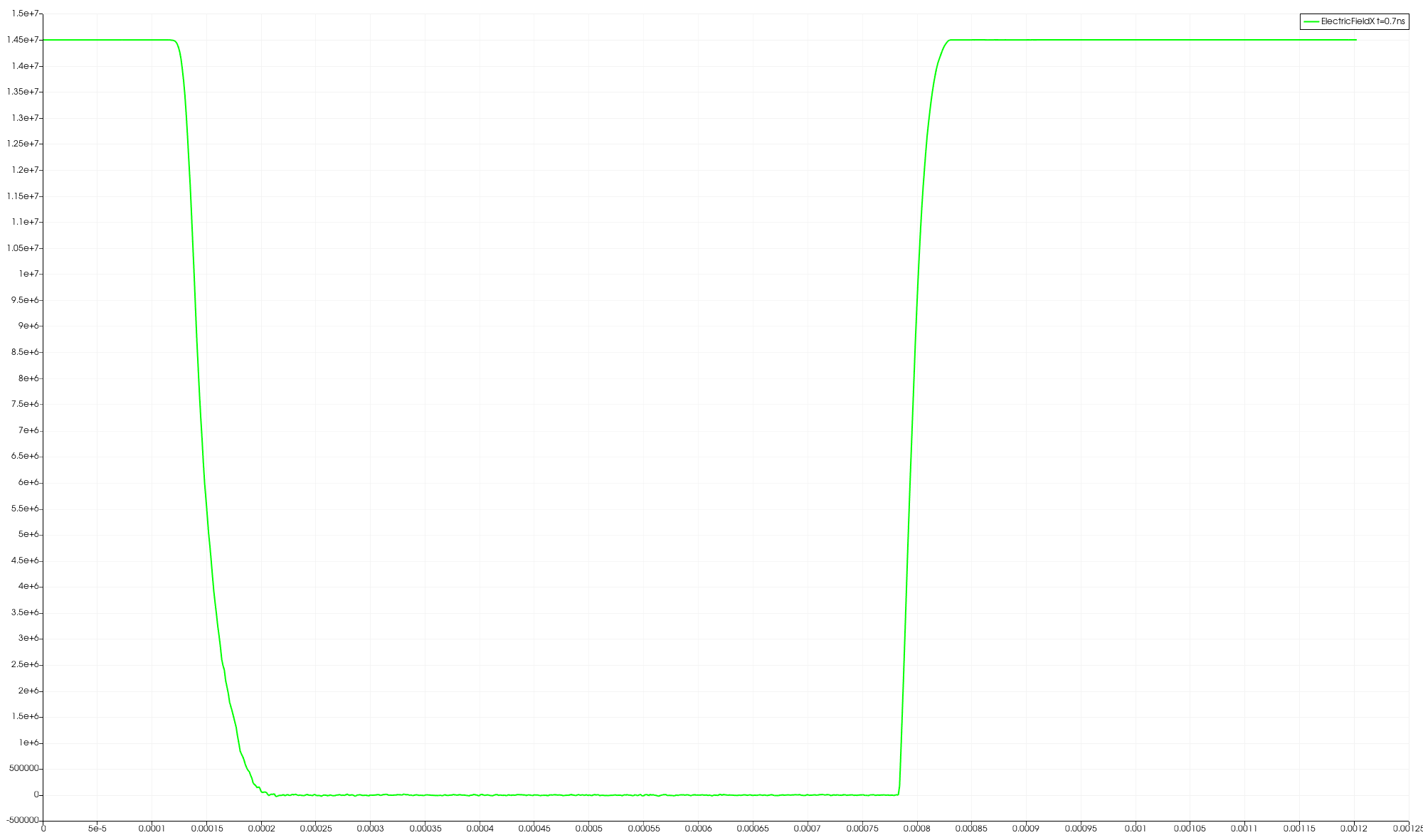
Fig. 7.10 Electric Field across the domain.
7.4.2.4. Cross-section Database
In this simulation setup, we have integrated a cross-section database that focuses solely on the effective and ionization cross sections from the LXCat database. These two categories of cross-sections are important because they dictate the formation rates and types of species that result from electron collision reactions with nitrogen gas. The effective cross-section represents the probability of any electron-induced reaction occurring, while the ionization cross-section specifically addresses the formation of electrons and N₂+ ions.
For our application in PICLas, we particularly need cross-section data for electron interactions with nitrogen gas molecules. This data was extracted from the LXCat database and converted into an accessible HDF5 format using a Python script located in the tools folder: piclas/tools/crosssection_database.
The resulting HDF5 file, XSec_Database_N2_Ionized.h5, referenced in the parameter.ini file, contains energy-dependent cross-section values. These values indicate the specific energies at which effective and ionization collisions occur, providing critical data for predicting species formation due to these interactions.
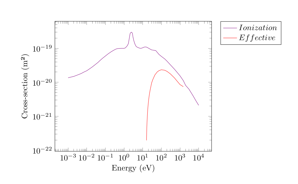
Fig. 7.11 Cross-section data for electron interactions with nitrogen (N₂) relevant to negative streamer development, depicting effective and ionization cross-sections across electron energy levels. These values are essential for modeling electron impact ionization and excitation processes in nitrogen, influencing the formation and propagation of negative streamers.
7.4.3. Comparison of Electron Fluid and PIC-MCC
In this tutorial, the negative streamer discharge was simulated using two different approaches.
In the first case, a hybrid Drift-Diffusion (DD) method was employed, in which electrons were modeled as a fluid, while ions were treated kinetically as particles. The fluid model for the electrons is a classical first-order model, which considers only the first moment of the distribution function (i.e., the density). In other words, this first-order approach accounts solely for changes in electron density based on drift and diffusion processes. No additional energy transport or equation is included.
In the second case, a fully kinetic PIC-MCC (Particle-in-Cell with Monte Carlo Collisions) simulation was performed, where both ions and electrons were treated kinetically as particles. This approach is naturally much more computationally demanding, as the total effort scales not only with the number of cells but also with the number of particles. Consequently, the DD simulation is approximately 12 times faster than the PIC-MCC simulation.
The following figures compare the results from both simulation methods. It is clearly visible that the streamer front propagates faster in the PIC-MCC simulation, as it is closer to the left boundary at time t=0.7ns. A similar behavior was also observed by Markosyan et al. [38], whose work this tutorial is based on. Markosyan et al. additionally simulated a second-order DD method, in which not only the first moment (density) but also the electron energy equation was taken into account.
In their second-order DD case, the streamer front also propagated significantly faster and was in better agreement with the PIC-MCC results. It is important to note that, in contrast to the hybrid approach used in this tutorial, Markosyan et al. applied a pure fluid model, in which ions were also treated as a fluid.
For future work, the DD implementation in PICLas should be extended to a second-order model. This would enable fast yet accurate streamer simulations compared to the fully kinetic PIC-MCC approach.
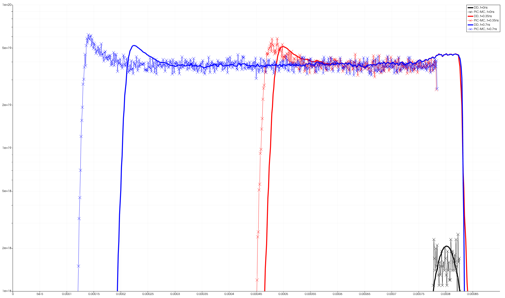
Fig. 7.12 Electron Density
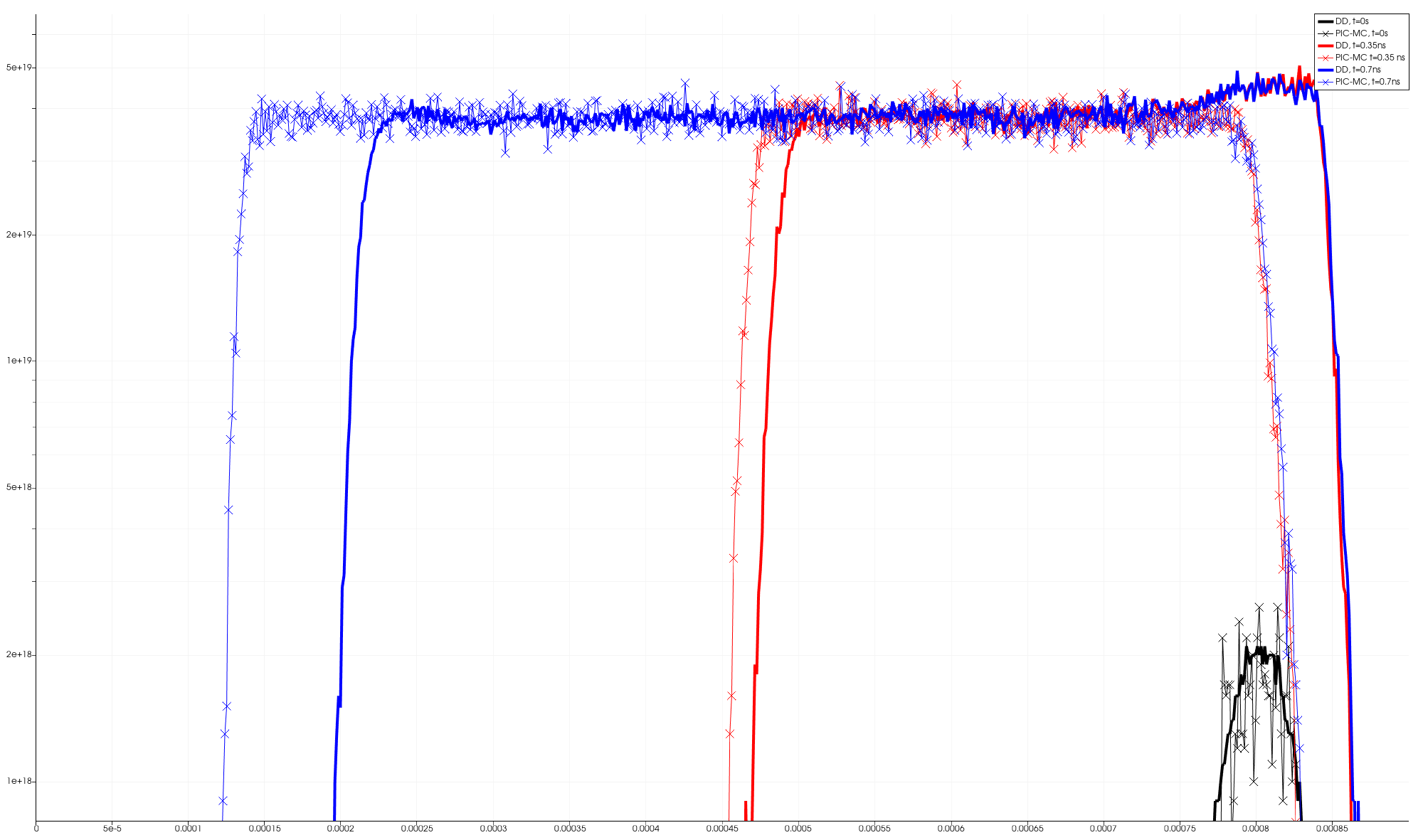
Fig. 7.13 Ion Density
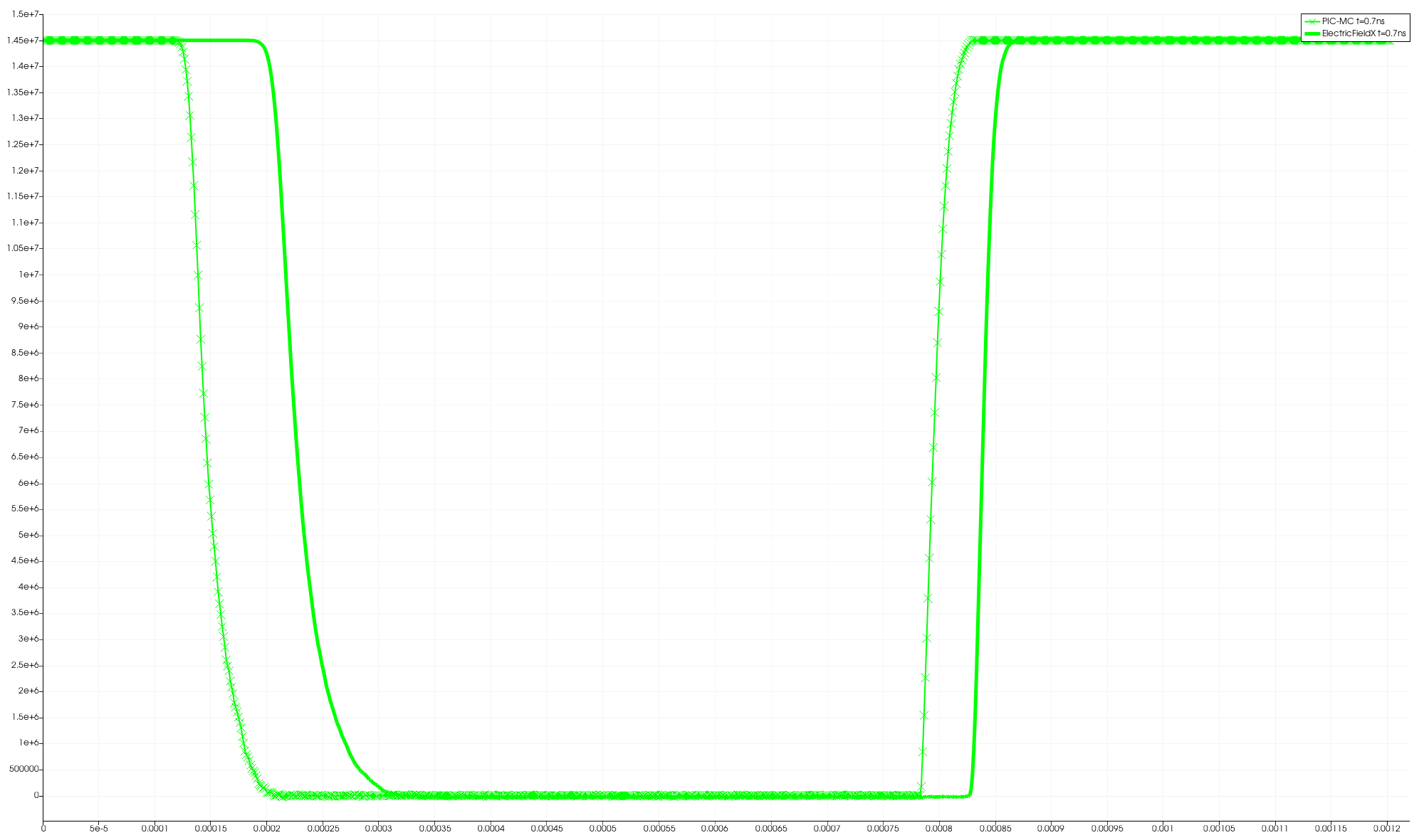
Fig. 7.14 Electric Field